
Natural Language Generation Background
Image courtesy of medium.com
These blog posts will focus on the problem of Natural Language Generation (NLG). Over various blog posts, we will explore key models that have significantly advanced the field, along with an exploration of some important problems that are trying to be solved in NLG.
This blog post will focus on the Natural Language Processing (NLP) and Deep Learning (DL) background required to understand the rest of the blog posts. However, due to the extensive nature of these topics, we will assume some background knowledge in order for us to focus on the NLG-specific aspects of DL. Specifically, we will assume that readers is familiar with
- What it means to train a DL model
- What regularization means
- Overfitting and underfitting
- Neural network basics: feed-forward neural networks, activation functions, backpropagation basics
For those without this background, we recommend the free Deep Learning book written by pioneers in this field, as well as these deep learning tutorials with popular frameworks like Tensorflow, PyTorch, and Keras.
Table of Contents
- Natural Language Processing
- Deep Learning
- References
Natural Language Processing
Natural Language Processing (NLP for short) is a broad term used to describe Machine Learning/Artificial Intelligence techniques for understanding language. The name of the area is a bit of a misnomer since some people recognize three broad areas that NLP has:
- Natural Language Processing (NLP): How do we process “human-understandable” language into “machine-understandable” input
- Natural Language Generation (NLG): How can we use machines to generate sensible speech and text
- Natural Language Understanding (NLU): How can we make machine understand what we mean when we communicate
Note that most problems end up having overlaps between the three areas, with NLP being quite necessary for the other two. For instance, it is hard for a machine to understand language if it is not able to first process it.
Language Models
In order for us to understand NLG, we often resort to a mathematical understanding of how language can be generated. Specifically, a language model is a way of modeling probability of a word or sequence of words. For instance, if we want to model how likely the phrase “did nothing wrong”, we would write down the probability as
Often, we want to model word and sentence probability with added conditions. For instance, if we wanted get the likely of the phrase “Thanos did nothing wrong” given that the previous word was “Thanos”, then that probability would be
N-grams
Given that sentences can be quite long (Gabriel García Márquez famously wrote a two-page long sentence in One Hundred Years of Solitude), it is often useful to just look at a subset of that sequence. To that end, we use n-grams (Cavnar and Trenkle 1994) which basically ask the question: given the previous n-1 words, what is the probability of the n-th word? In probability terms, this looks like
Skip-grams
N-grams are limited by the sequential nature of the n-gram; you are using as context the n-1 words before the n-th word and only those. A more flexible approach has been skip-grams (Guthrie et al. 2006) which still will use some n number of words as context, but it allows you to skip over some words. Skipgrams will end up choosing the words that are the most significant of the sentence. For instance, when predicting the word following the sentence “The dog happily ate the “ and we choose to have n=2, we might choose the words [“dog”, “ate”] rather than having to focus solely on the words [“ate”, “the”] since “dog” and “ate” tell us more useful information.
Forward and Backward Probabilities
So far, we have seen probabilities of the next word given previous words. These types of probabilities are called forward probabilities.
However, we can also look at backward probabilities, meaning the probability of a past word given the current words.
Though not as useful for predicting future words, they are still useful for understanding sequences and obtaining features for the context surrounding words (Peters et al. 2018).
Word Representations
Word representations are ways of representing words in a machine-understandable way; the most common way of doing so is by representing a word as a vector. They are especially useful for ML algorithms since the vector representation allows for statistical methods to be used, especially optimization-based algorithms.
As an example, suppose we wanted to represent the sentence “The dog is the goodest of boys”. One way we could do it is by using bag-of-words representations. Suppose our entire dictionary consisted of the words [the, dog, is, bad, goodest, of, boys, great]. Then, the sentence would look as follows
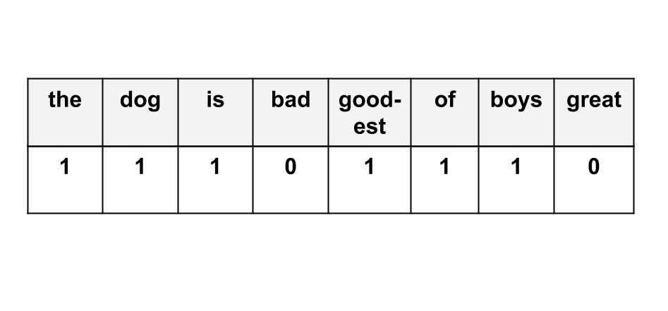
Example of bag-of-words representation of sentence “The dog is the goodest of boys”
Here, we define a dimension for each word and the vector for a word will have a 1 if that word is present, 0 otherwise.
The sentence “The dog is good” would look like
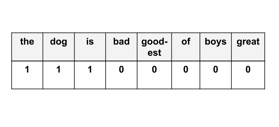
Example of bag-of-words representation of sentence “The dog is good”
Note that since we did not include “good” in our original dictionary, this does not appear in our vector.
Distributed Word Representations
There are multiple types of word representations, such as those based on clustering, one-hot encodings, and based on co-occurrences (the article here explains a lot of different types of word representations quite well). However, as we saw in the previous example, a big problem is the sparsity of the space (meaning that we have too many dimensions for too few data points) and that we might not handle unseen words well (i.e. we are unable to generalize).
Among the many different kinds of word representations, the one that has gained the most traction over the past few years is distributed word representations (also called word embeddings). These use condensed feature vectors in latent spaces that are not immediately human-understandable. This means that we can generalize to unseen words and the problem of sparsity is handled better. Deep Learning is often used with these (Turian, Ratinov, and Bengio 2010).
For instance, we could run a neural network on the sentence “the dog is good” and get a latent space encoding.
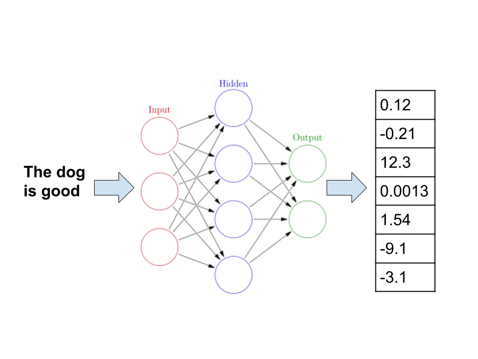
Word embeddings example
Though we might not be able to easily understand what these dimensions mean in terms of human terms, they are often more useful for machine learning algorithms.
Deep Learning
Within Machine Learning (ML), the area that has spearheaded a lot of the performance gains has been Deep Learning (DL). DL is the area of ML that deals with neural networks, which allow models to automatically learn latent features from data. In this section, we will cover some of the aspects of deep learning that have been widely used in NLP.
Residual Networks
Residual networks have been used quite widely for some time now (Szegedy et al. 2017) with a lot of recent architectures (such as ELMo and BERT) using these and with most state-of-the-art using these by default.
The main idea is that we have some “skip-ahead” connections in the neural architecture.
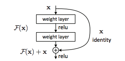
Image from https://miro.medium.com/max/651/0sGlmENAXIZhSqyFZ*
There are two main ideas that motivate residual connections:
- “Short-circuit” connections: A key hyperparameter in neural architectures is the number of layers, with the trend being that more is better. However, for some instances it is not necessary to have that many layers. To alleviate some of the hyperparameter tuning work, residual connections can help give the network the ability to decide to use all layers or to ignore some of them.
- “Refresh memory”: The other big idea is that by having some connections that skip layers, we can give the deeper layers of the network a refresher on what the original input looked like. That way, the network can used the latent features along with the original ones.
For more information on residual neural networks, check out this tutorial.
Convolutional Neural Networks
Arguably, the first networks that really impressed the world (LeCun and Bengio 1995) are convolutional neural networks (CNN). The distinguishing feature of CNN’s are convolutional layers, which take into account an input’s neighboring values. In other words, rather than looking at each component of the input vector as “independent”, they look at each component’s neighborhood.
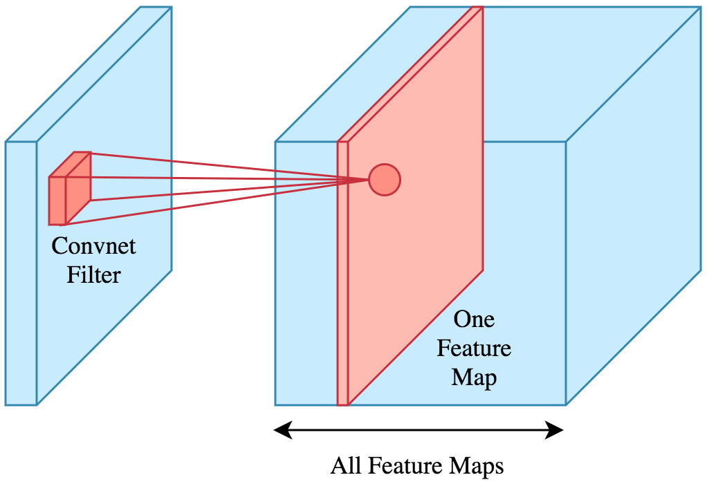
Image from https://www.kdnuggets.com/2019/07/convolutional-neural-networks-python-tutorial-tensorflow-keras.html
So, a CNN ends up with convolutional layers at the beginning and then some “regular” network connections at the end. Though CNN’s are often associated with image inputs, they can also be used in sequential data. For instance, we could look at the window of 2 words before and after our current word.
For a more in-depth tutorial into CNN’s, there are multiple online resources; this tutorial by kdnuggets is quite good.
Recurrent Neural Networks
Recurrent Neural Networks (RNN’s) deal with an important limitation of CNN’s: their fixed-size window. CNN’s convolutions have a fixed window that they deal with and they have a fixed sized input that they can deal with. This is problematic for sequences such as sentences since often vary in length.
RNN’s can deal with this by introducing a special layer called the Recurrent layer. These use cells that take as input a part of the sequence and the output of the cell with the previous input
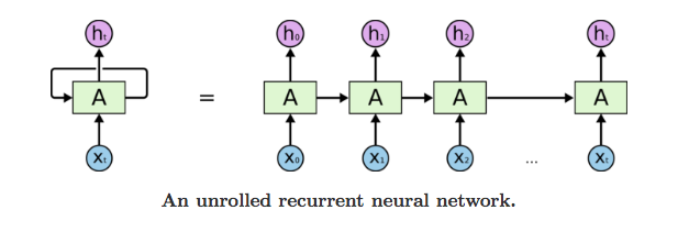
Image from https://miro.medium.com/max/941/1go8PHsPNbbV6qRiwpUQ5BQ.png*
Given this set up, it is easy to see how these could be used for language modeling since they can (theoretically) take into account as many previous words as possible (Mikolov et al. 2010).
To learn more about RNN’s check out this tutorial.
LSTM Cells
Normal RNN’s face various limitations, the most glaring being that it might be difficult to train them due to exploding/vanishing gradients and they can have trouble remembering long sequences.
Rather than using RNN’s, what people end up using is often Long Short-Term Memory Cells (LSTM Cells). The details of LSTM cells are quite intricate (Gers, Schmidhuber, and Cummins 1999), yet the intuition behind these is remarkably simple: LSTM’s can have longer term memory by choosing what to remember and what to forget.
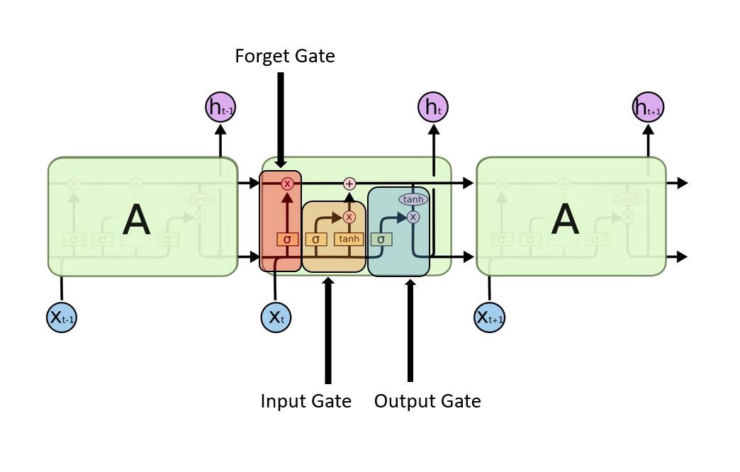
Image from https://miro.medium.com/max/1566/1MwU5yk8f9d6IcLybvGgNxA.jpeg*
To learn more about LSTM’s check out this tutorial.
Bidirectional RNNs
RNN’s are usually used for future prediction, meaning that you follow the “forward” probability Language Model. However, they can also be used to model the backward probabilities.
The rationale behind this seems a bit unintuitive: why would you want to predict what has already happened? And often, you don’t actually want to predict what has happened (and you can’t use them to predict the future since that is not what you’re learning). The main reason why you would use them is for understanding the entire sequence rather than trying to predict future incidents.
This reasoning motivates Bidirectional RNN’s (Schuster and Paliwal 1997), which use both forward and backward Language Models.
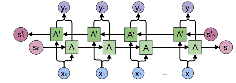
Image from https://miro.medium.com/max/1146/16QnPUSv_t9BY9Fv8_aLb-Q.png*
To learn more about bi-RNN’s check out this tutorial.
Encoder-Decoder Networks (seq2seq)
This seq2seq architecture was introduced in 2014 by (Sutskever et al., 2014) in an effort to produce better translations between languages. These types of networks are composed of two parts: an encoder and a decoder. The encoder is a neural network that takes the input (in NLP this might be a sequence of words) and runs it through the network to produce a simpler representation in a new vector space. The decoder, also a neural network, then takes a vector from this new space, and translates it into another vector space.
For example, consider the problem of translating between languages such as converting an English sentence to Spanish. The encoder network, once trained, would be able to encode the English sentence in a new, intermediate representation that captures the semantics of the English sentence. Then, the decoder network would take this intermediate representation that contains the meaning of the original sentence, and converts it to an equivalent sentence in Spanish.
Attention Mechanisms
Intuitively, we know that certain parts of a sentence or sequence are more important than others. As humans, we can do this fairly easily by remembering what we have previously seen. However, this can be difficult for computers that lack the complex memory and reasoning skills that are built into the human brain. This is where attention mechanisms come into play. These help identify which parts of a sequence are most important, and keep track of them as the model continues to process new information.
Furthermore, there are many words that have a different meaning depending on the context in which they are used. This phenomenon is called polysemy. For instance, take the following sentence:
It is a mole.
Depending on the context, I could mean either that “it” is a small, burrowing mammal, or that “it” is a dark blemish on the skin, or even that “it” is an undercover spy. Attention mechanisms allow for neural networks to keep track of important words that might clue it in what “it” is actually referring to.
Each word in an input sequence is assigned a score based on its context, i.e. the surrounding words. This attention score can be computed in many different ways, and some prominent ways of doing so are listed in the following table:
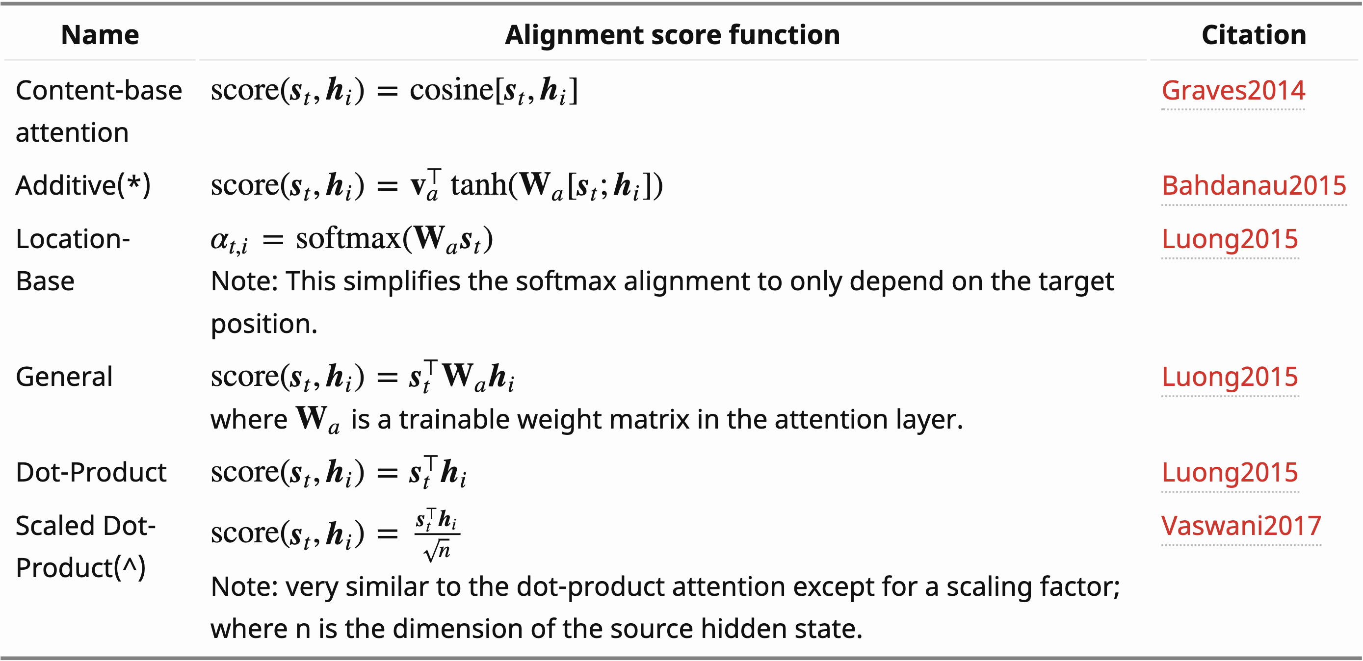
Table of attention mechanisms from https://lilianweng.github.io/lil-log/2018/06/24/attention-attention.html
In the above table, st is a vector representing the hidden state in the decoder for the word at position t, and hi is a vector created by concatenating the forward hidden states with the backward hidden states of the recurrent unit for the word at position i. For a more in-depth history of attention mechanisms, we recommend this excellent blog post by Lilian Weng.
Example: Bahdanau’s Attention Mechanism
Attention mechanisms were introduced into typical encoder-decoder architectures as a means of keeping track of the important parts of the input sequence. This was first done in the context of natural language processing, more specifically machine translation (Bahdanau et al., 2014). They add an attention mechanism, which they call the alignment model, to the decoder.
The encoder is a bidirectional LSTM that maps the input sequence to a series of annotations. An annotation is vector that is the result of concatenating the forward hidden states with the backwards hidden states. Put more simply, it is just a representation of the word along with some of the context surrounding it. Each annotation contains information about the whole input sequence with an emphasis on the words surrounding the $i^{th}$ word as a result of the tendency of LSTMs to better capture information about more recent input.
The decoder can then use these annotations to produce context vectors, which are a weighted sum of the annotations for words in the current sequence:
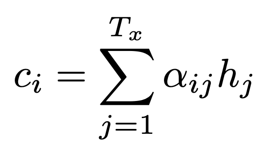
where Ci is a context vector and hj is an annotation. The weights of the annotations $\alpha$ij for this summation are found by
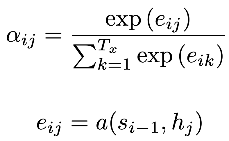
where eij is the alignment model, which provides a score of how well the input around position j and the output at position i match, and si-1 is the RNN hidden state, which provides a representation of all previous input.
The alignment is basically the importance of a given annotation in producing the current output word. The alignment function is itself a feedforward neural network that is trained alongside the overall encoder-decoder model.
These context vectors are fed into later layers of the decoder in order to eventually predict the output sequence that is associated with the input sequence. In this way, we can use attention mechanisms for a variety of natural language processing tasks, including better predicting how to translate sentences between languages, or predicting the next word in a given sequence.
Transformers
One recent major breakthrough in natural language processing is the transformer network. This is a deep neural network model that can be used as a way to understand sequential data without recurrence or convolutions and instead uses only attention mechanisms in its architecture. This was first introduced by a team of researchers at Google in 2017 (Vaswani et al., 2017), and they use what is called the self-attention mechanism instead of recurrent units to keep track of associations and correlations in the input.
These networks were originally developed to solve the problem of sequence transduction, which is transforming one input type to another. Often, this is done for tasks in machine translation or converting text to speech. Overall, this model does a good job at these tasks, so let’s dive into some specifics to get a better understanding of why.
Architecture
As described in the original paper, the architecture of a transformer network follows the same encoder-decoder structure, with multiple layers in each.
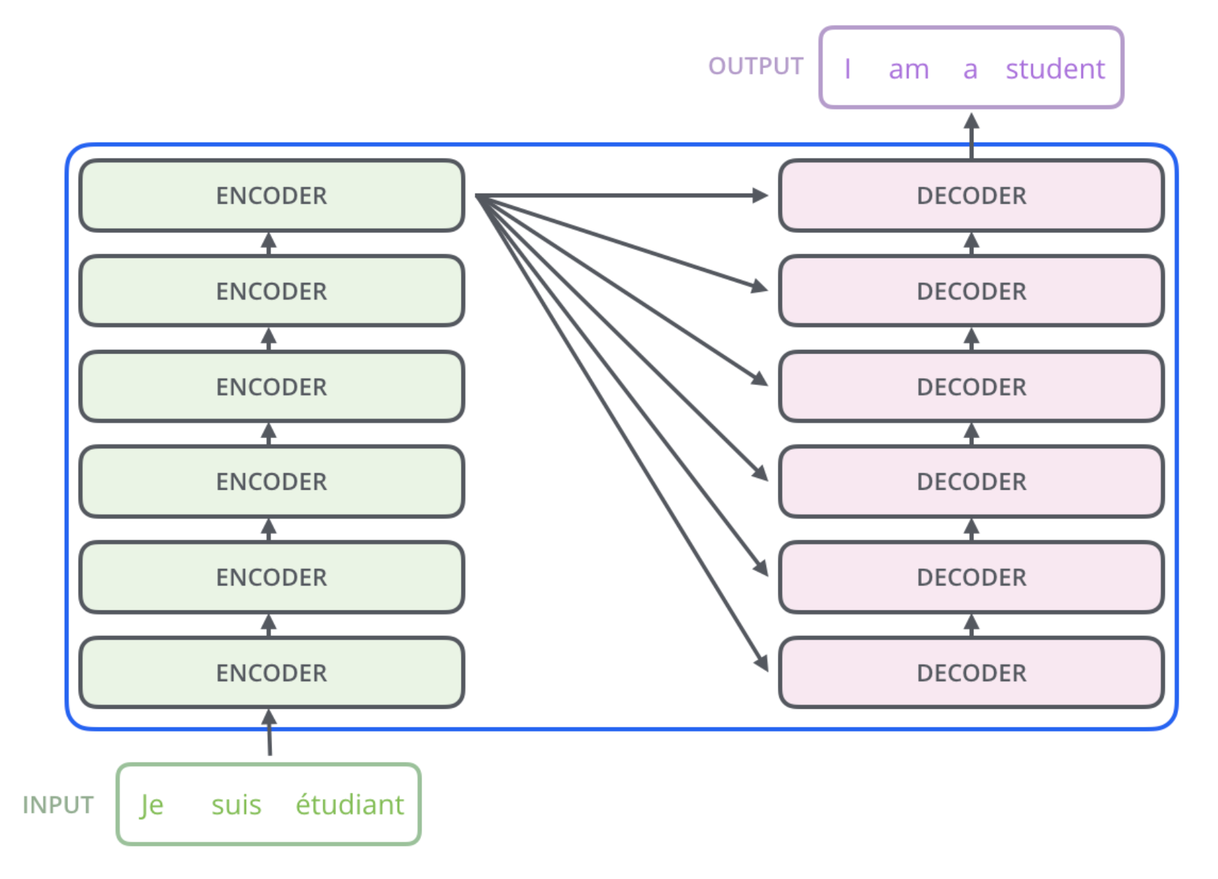
High level architecture of a transformer. From http://jalammar.github.io/illustrated-transformer/
Each encoder layer consists of a self-attention layer and a feed forward network.
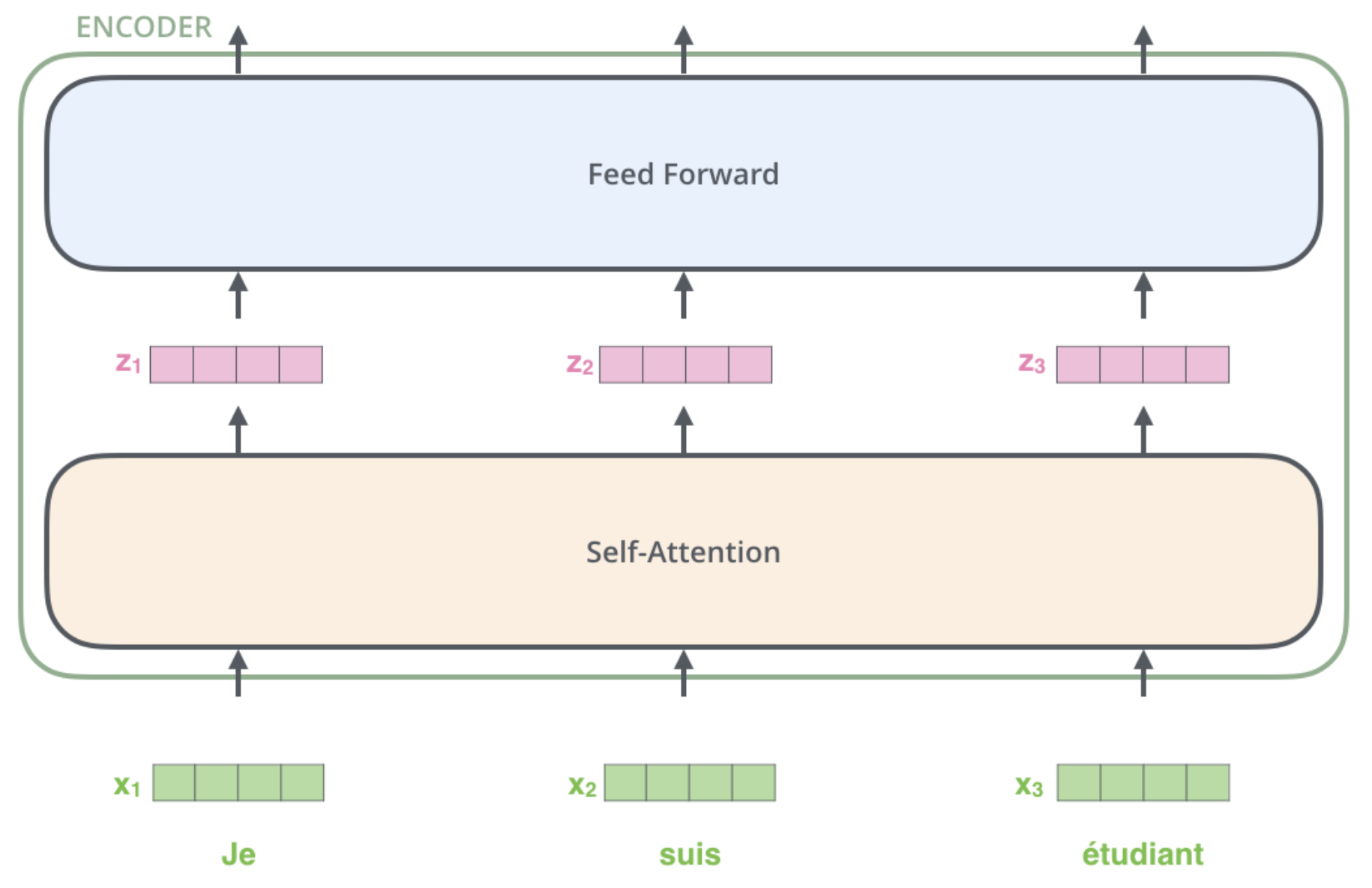
High level architecture of an encoder layer in a transformer. From http://jalammar.github.io/illustrated-transformer/
The decoder layers are very similar. They also have the self-attention layer and a feed forward network, but have an additional attention layer in between to aid in the decoding process.
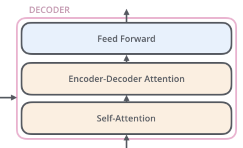
High level architecture of an decoder layer in a transformer. From http://jalammar.github.io/illustrated-transformer/
The encoder-decoder attention mechanism used here is one that mimics one of the previously discussed attention mechanisms that was used in a regular encoder-decoder network, such as the one from (Bahdanau et al., 2015). This allows the decoder layer to look at all positions of the input sequence.
Self-Attention Mechanism
Self-attention is a technique that tries to produce a new representation of an input sequence by relating different positions in the sequence with other positions. This provides a way to encode correlations between words in a sentence, and allows the network to incorporate these relations into its processing. For example, as previously discussed, recurrent units in RNNs provide are one way to do this. This has previously been used in conjunction with LSTMs to improve the processing of sequential data in natural language understanding tasks (Cheng et al., 2016).
Scaled Dot-Product Attention
One of the key features of the transformer network introduced by Vaswani et al. was a new attention mechanism: Scaled Dot-Product Attention. This is very similar to dot-product attention (Luong et al., 2015), but they add a scale factor that is the dimension of the source hidden state. This effectively normalizes the value and helps prevent cases where the softmax function is pushed into spaces with small gradients, i.e. alleviating the vanishing gradient problem.
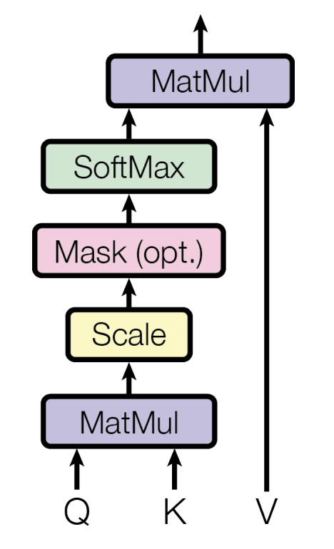
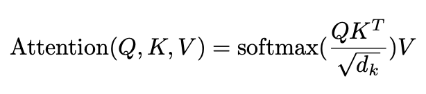
Scaled Dot-Product Attention from (Vaswani et al., 2017)
The inputs here are the query, key, and value vectors (note: In the paper, multiple queries, keys, and values are processed simulataneously and are thus packed into matrices). We start with a word in the input sequence and calculate a word embedding for it in order to get a vector representation of the word. Then, there is a separate transformation matrix that is used to convert these word embeddings to the proper space of queries, keys, and values. These weights/values in these transformation matrices are found during the training process. The intuition here is once again that this attention mechanism will produce a new representation of the input sequence in order to determine how well the words are correlated with each other.
Multi-Head Attention
Additionally, they use multi-head attention in order to allow the transformer model to “attend to information from different representation subspaces at different positions.” This is also done as an optimization for the model, as it allows for the attention function to be computed mutliple times in parallel.
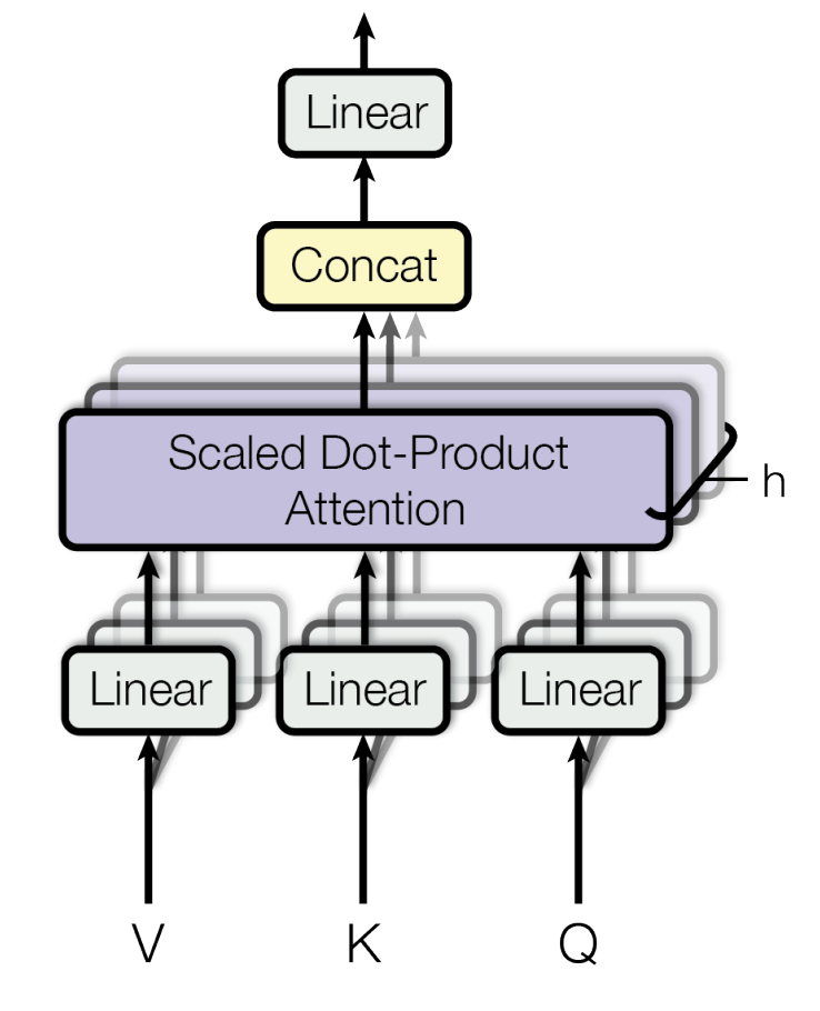
Multi-Head Attention Mechanism from (Vaswani et al., 2017)
Further Reading on Transformers
For more a more in-depth discussion of the specifics of how transformers work, we recommend this blog post by Jay Allamar.
For those who are interested in digging into the details of how to implement one of these transformer networks, this excellent article from Harvard’s NLP group provides a walkthrough of a fully functioning Python implementation.
References
- Bahdanau, Dzmitry, Kyunghyun Cho, and Yoshua Bengio. “Neural machine translation by jointly learning to align and translate.” arXiv preprint arXiv:1409.0473 (2014).
- Cavnar, William B., and John M. Trenkle. “N-gram-based text categorization.” In Proceedings of SDAIR-94, 3rd annual symposium on document analysis and information retrieval, vol. 161175. 1994.
- Cheng, Jianpeng, Li Dong, and Mirella Lapata. “Long short-term memory-networks for machine reading.” arXiv preprint arXiv:1601.06733 (2016).
- Gers, Felix A., Jürgen Schmidhuber, and Fred Cummins. “Learning to forget: Continual prediction with LSTM.” (1999): 850-855.
- Guthrie, David, Ben Allison, Wei Liu, Louise Guthrie, and Yorick Wilks. “A closer look at skip-gram modelling.” In LREC, pp. 1222-1225. 2006.
- LeCun, Yann, and Yoshua Bengio. “Convolutional networks for images, speech, and time series.” The handbook of brain theory and neural networks 3361, no. 10 (1995): 1995.
- Luong, Minh-Thang, Hieu Pham, and Christopher D. Manning. “Effective approaches to attention-based neural machine translation.” arXiv preprint arXiv:1508.04025 (2015).
- Mikolov, Tomáš, Martin Karafiát, Lukáš Burget, Jan Černocký, and Sanjeev Khudanpur. “Recurrent neural network based language model.” In Eleventh annual conference of the international speech communication association. 2010.
- Peters, Matthew E., Mark Neumann, Mohit Iyyer, Matt Gardner, Christopher Clark, Kenton Lee, and Luke Zettlemoyer. “Deep contextualized word representations.” arXiv preprint arXiv:1802.05365 (2018).
- Schuster, Mike, and Kuldip K. Paliwal. “Bidirectional recurrent neural networks.” IEEE Transactions on Signal Processing 45, no. 11 (1997): 2673-2681.
- Sutskever, I., O. Vinyals, and Q. V. Le. “Sequence to sequence learning with neural networks.” Advances in NIPS (2014).
- Szegedy, Christian, Sergey Ioffe, Vincent Vanhoucke, and Alexander A. Alemi. “Inception-v4, inception-resnet and the impact of residual connections on learning.” In Thirty-First AAAI Conference on Artificial Intelligence. 2017.
- Turian, Joseph, Lev Ratinov, and Yoshua Bengio. “Word representations: a simple and general method for semi-supervised learning.” In Proceedings of the 48th annual meeting of the association for computational linguistics, pp. 384-394. Association for Computational Linguistics, 2010.
- Vaswani, Ashish, et al. “Attention is all you need.” Advances in neural information processing systems. 2017.